Like many of you, I love ggplot2. The ability to make beautiful, informative plots quickly is a major boon to my research workflow. One plot I’ve been particularly fond of recently is the ‘violin + boxplot + jittered dataset’ combo, which nicely provides an overview of the raw data, the probability distribution, and ‘statistical inference at a glance’ via medians and confidence intervals. However, as pointed out in this tweet by Naomi Caselli, violin plots mirror the data density in a totally uninteresting/uninformative way, simply repeating the same exact information for the sake of visual aesthetic. Not to mention, for some at least they are actually a bit lewd. In my quest for a better plot, which can show differences between groups or conditions while providing maximal statistical information, I recently came upon the ‘split violin’ plot. This nicely deletes the mirrored density, freeing up room for additional plots such as boxplots or raw data. Inspired by a particularly beautiful combination of split-half violins and dotplots, I set out to make something a little less confusing. In particular, dot plots are rather complex and don’t precisely mirror what is shown in the split violin, possibly leading to more confusion than clarity. Introducing ‘elephant’ and ‘raincloud’ plots, which combine the best of all worlds! Read on for the full code-recipe plus some hacks to make them look pretty (apologies for poor markup formatting, haven’t yet managed to get markdown to play nicely with wordpress)!

Let’s get to the data – with extra thanks to @MarcusMunafo, who shared this dataset on the University of Bristol’s open science repository.

First, we’ll set up the needed libraries and import the data:

library(readr)
library(tidyr)
library(ggplot2)
library(Hmisc)
library(plyr)
library(RColorBrewer)
library(reshape2)

source(“https://gist.githubusercontent.com/benmarwick/2a1bb0133ff568cbe28d/raw/fb53bd97121f7f9ce947837ef1a4c65a73bffb3f/geom_flat_violin.R”)

my_data<-read.csv(url(“https://data.bris.ac.uk/datasets/112g2vkxomjoo1l26vjmvnlexj/2016.08.14_AnxietyPaper_Data%20Sheet.csv”))

head(X)

Although it doesn’t really matter for this demo, in this experiment healthy adults recruited from MTurk (n = 2006) completed a six alternative forced choice task in which they were presented with basic emotional expressions (anger, disgust, fear, happiness, sadness and surprise) and had to identify the emotion presented in the face. Outcome measures were recognition accuracy and unbiased hit rate (i.e., sensitivity).

For this demo, we’ll focus on the unbiased hitrate for anger, disgust, fear, and happiness conditions. Let’s reshape the data from wide to long format, to facilitate plotting:

library(reshape2)
my_datal <- melt(my_data, id.vars = c(“Participant”), measure.vars = c(“AngerUH”, “DisgustUH”, “FearUH”, “HappyUH”), variable.name = “EmotionCondition”, value.name = “Sensitivity”)

head(my_datal)

Now we’re ready to start plotting. But first, lets define a theme to make pretty plots.

raincloud_theme = theme(
text = element_text(size = 10),
axis.title.x = element_text(size = 16),
axis.title.y = element_text(size = 16),
axis.text = element_text(size = 14),
axis.text.x = element_text(angle = 45, vjust = 0.5),
legend.title=element_text(size=16),
legend.text=element_text(size=16),
legend.position = “right”,
plot.title = element_text(lineheight=.8, face=”bold”, size = 16),
panel.border = element_blank(),
panel.grid.minor = element_blank(),
panel.grid.major = element_blank(),
axis.line.x = element_line(colour = ‘black’, size=0.5, linetype=’solid’),
axis.line.y = element_line(colour = ‘black’, size=0.5, linetype=’solid’))

Now we need to calculate some summary statistics:

lb <- function(x) mean(x) – sd(x)
ub <- function(x) mean(x) + sd(x)

sumld<- ddply(my_datal, ~EmotionCondition, summarise, mean = mean(Sensitivity), median = median(Sensitivity), lower = lb(Sensitivity), upper = ub(Sensitivity))

head(sumld)

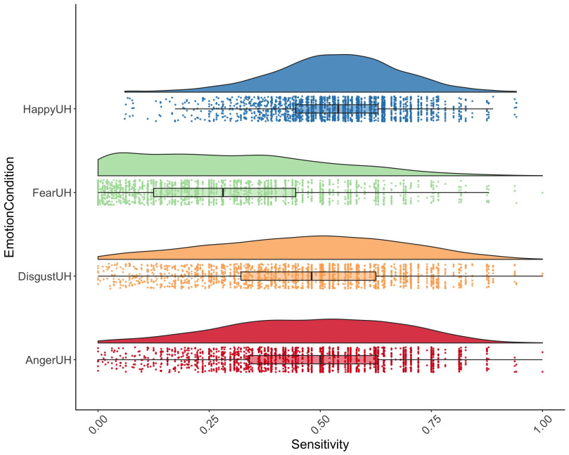
Now we’re ready to plot! We’ll start with a ‘raincloud’ plot (thanks to Jon Roiser for the great suggestion!):

g <- ggplot(data = my_datal, aes(y = Sensitivity, x = EmotionCondition, fill = EmotionCondition)) +
geom_flat_violin(position = position_nudge(x = .2, y = 0), alpha = .8) +
geom_point(aes(y = Sensitivity, color = EmotionCondition), position = position_jitter(width = .15), size = .5, alpha = 0.8) +
geom_boxplot(width = .1, guides = FALSE, outlier.shape = NA, alpha = 0.5) +
expand_limits(x = 5.25) +
guides(fill = FALSE) +
guides(color = FALSE) +
scale_color_brewer(palette = “Spectral”) +
scale_fill_brewer(palette = “Spectral”) +
coord_flip() +
theme_bw() +
raincloud_theme

g

I love this plot. Adding a bit of alpha transparency makes it so we can overlay boxplots over the raw, jittered data points. In one https://blogs.scientificamerican.com/literally-psyched/files/2012/03/ElephantInSnake.jpegplot we get basically everything we need: eyeballed statistical inference, assessment of data distributions (useful to check assumptions), and the raw data itself showing outliers and underlying patterns. We can also flip the plots for an ‘Elephant’ or ‘Little Prince’ Plot! So named for the resemblance to an elephant being eating by a boa-constrictor:

g <- ggplot(data = my_datal, aes(y = Sensitivity, x = EmotionCondition, fill = EmotionCondition)) +
geom_flat_violin(position = position_nudge(x = .2, y = 0), alpha = .8) +
geom_point(aes(y = Sensitivity, color = EmotionCondition), position = position_jitter(width = .15), size = .5, alpha = 0.8) +
geom_boxplot(width = .1, guides = FALSE, outlier.shape = NA, alpha = 0.5) +
expand_limits(x = 5.25) +
guides(fill = FALSE) +
guides(color = FALSE) +
scale_color_brewer(palette = “Spectral”) +
scale_fill_brewer(palette = “Spectral”) +

coord_flip() +

theme_bw() +
raincloud_theme

For those who prefer a more classical approach, we can replace the boxplot with a mean and confidence interval using the summary statistics we calculated above. Here we’re using +/- 1 standard deviation, but you could also plot the SEM or 95% CI:

g <- ggplot(data = my_datal, aes(y = Sensitivity, x = EmotionCondition, fill = EmotionCondition)) +
geom_flat_violin(position = position_nudge(x = .2, y = 0), alpha = .8) +
geom_point(aes(y = Sensitivity, color = EmotionCondition), position = position_jitter(width = .15), size = .5, alpha = 0.8) +
geom_point(data = sumld, aes(x = EmotionCondition, y = mean), position = position_nudge(x = 0.3), size = 2.5) +
geom_errorbar(data = sumld, aes(ymin = lower, ymax = upper, y = mean), position = position_nudge(x = 0.3), width = 0) +
expand_limits(x = 5.25) +
guides(fill = FALSE) +
guides(color = FALSE) +
scale_color_brewer(palette = “Spectral”) +
scale_fill_brewer(palette = “Spectral”) +
theme_bw() +
raincloud_theme

g

Et voila! I find that the combination of raw data + box plots + split violin is very powerful and intuitive, and really leaves nothing to the imagination when it comes to the underlying data. Although here I used a very large dataset, I believe these would still work well for more typical samples sizes in cognitive neuroscience (i.e., N ~ 30-100), although you may want to only include the boxplot for very small samples.

I hope you find these useful, and you can be absolutely sure they will be appearing in some publications from our workbench as soon as possible! Go forth and make it rain!

Thanks very much to @naomicaselli, @jonclayden, @patilindrajeets, & @jonroiser for their help and inspiration with these plots!